
How To Freeze Multiple Panes In Excel
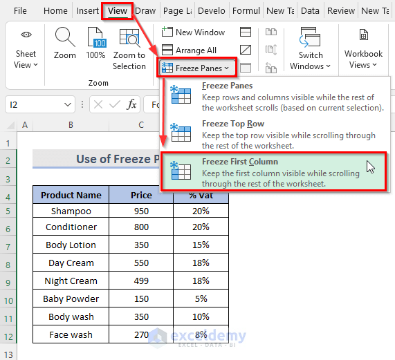
How To Freeze Multiple Panes In Excel - For example, if you want to freeze the first three rows, select the fourth row. In this example, cell c4 is selected which means rows 1:3 and columns a:b will be frozen and stay anchored at the top and to the left of the sheet. Web select the third column. Select view > freeze panes > freeze panes. Web go to the view tab.
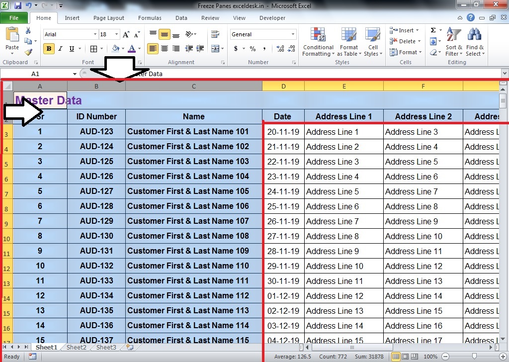
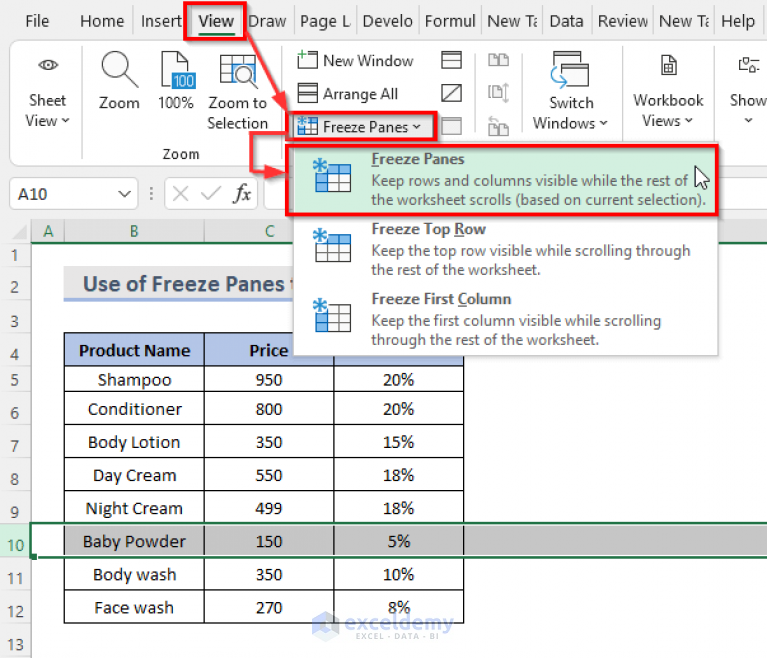
Web in your spreadsheet, select the row below the rows that you want to freeze. You can also select row 4 and press the alt key > w > f > f. Select a cell that is below the rows and right to the columns we want to freeze. Web select the third column. This will launch many a menu of options. We selected cell d9 to freeze the product name and price up to day cream. Click the freeze panes option.
How to freeze multiple panes in excel 2016 dasing
On the view tab > window > unfreeze panes. Select view > freeze panes > freeze panes. Web go to the view tab > freezing panes. Web select the third column. Users can also choose to freeze multiple rows or columns by selecting the appropriate cells before choosing to freeze panes. Web on the view.
How to Freeze Panes in Excel YouTube
Web go to the view tab > freezing panes. After you have frozen rows and / or columns, you will not be able to scroll up to the top of the worksheet. This will launch many a menu of options. Web select the third column. Web go to the view tab. Web to freeze multiple.

How to freeze panes across multiple Excel worksheets Spreadsheet Vault
Select view > freeze panes > freeze panes. For example, to freeze top two rows in excel, we select cell a3 or the entire row 3, and click freeze panes: On the view tab > window > unfreeze panes. To unfreeze panes, tap view > freeze panes, and then clear all the selected options. Select.
The Most Usefulness Of Freeze Panes In MSExcel 21's Secret
The row (s) and column (s) will be frozen in place. Select the view tab from the ribbon. Web go to the view tab. Excel freezes the first 3 rows. You can also select row 4 and press the alt key > w > f > f. Web the basic method for freezing panes in.
How to use Freeze Panes in Excel? How to Freeze Multiple Rows/Columns
Click the freeze panes option. We selected cell d9 to freeze the product name and price up to day cream. Choose the freeze panes option from the menu. You can also select row 4 and press the alt key > w > f > f. Excel freezes the first 3 rows. Select a cell that.

How to freeze multiple panes in excel dasthegreen
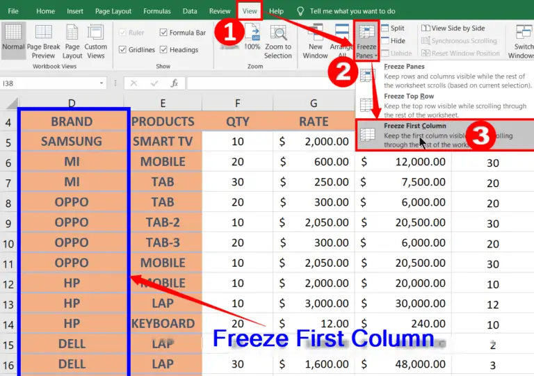
Web to freeze multiple columns (starting with column a), select the column to the right of the last column you want to freeze, and then tap view > freeze panes > freeze panes. Web go to the view tab > freezing panes. Web in your spreadsheet, select the row below the rows that you want.
How to Freeze Multiple Panes in Excel (4 Criteria) ExcelDemy
Web go to the view tab > freezing panes. Web to freeze multiple columns (starting with column a), select the column to the right of the last column you want to freeze, and then tap view > freeze panes > freeze panes. To unfreeze panes, tap view > freeze panes, and then clear all the.
How to Freeze Multiple Rows and or Columns in Excel using Freeze Panes
Web select the third column. We selected cell d9 to freeze the product name and price up to day cream. Click the freeze panes option. Click on the freeze panes command in the windows section of the ribbon. Excel freezes the first 3 rows. Select a cell that is below the rows and right to.
How to Freeze Multiple Rows and Columns in Excel using Freeze Panes
After you have frozen rows and / or columns, you will not be able to scroll up to the top of the worksheet. To unfreeze panes, tap view > freeze panes, and then clear all the selected options. Click on the freeze panes command in the windows section of the ribbon. We selected cell d9.
How to Freeze Multiple Panes in Excel (4 Criteria) ExcelDemy
Select view > freeze panes > freeze panes. To unfreeze panes, tap view > freeze panes, and then clear all the selected options. Web go to the view tab > freezing panes. Web go to the view tab. Select the cell below the rows and to the right of the columns you want to keep.
How To Freeze Multiple Panes In Excel Click the freeze panes option. Select a cell that is below the rows and right to the columns we want to freeze. Select the cell below the rows and to the right of the columns you want to keep visible when you scroll. We selected cell d9 to freeze the product name and price up to day cream. Web select the third column.
As The Result, You'll Be Able To Scroll Through The Sheet Content While Continuing To View The Frozen Cells In The First Two Rows:
Select the view tab from the ribbon. Web go to the view tab > freezing panes. Web select the third column. You can also select row 4 and press the alt key > w > f > f.
On The View Tab, In The Window Section, Choose Freeze Panes > Freeze Panes.
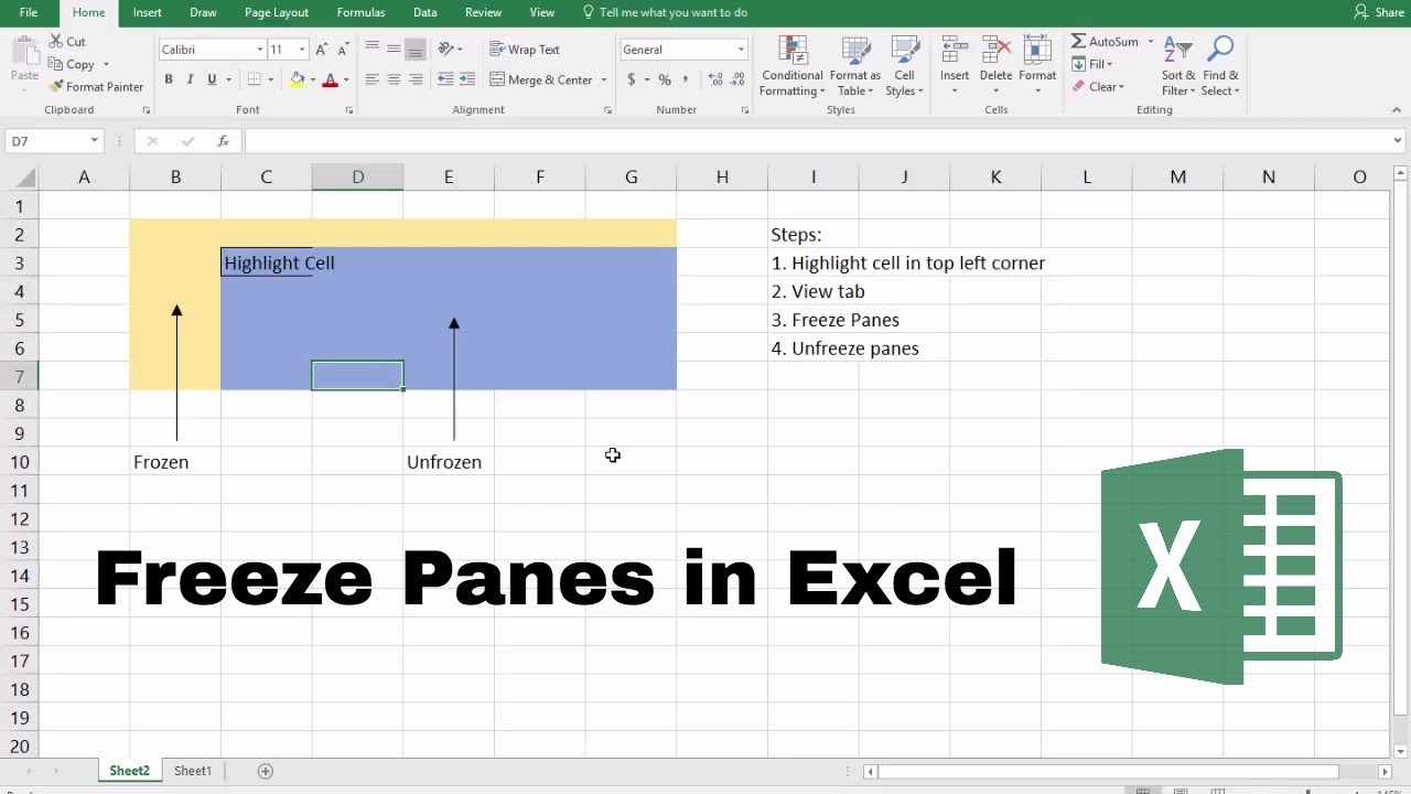
For example, if you want to freeze the first three rows, select the fourth row. Click on the freeze panes command in the windows section of the ribbon. Web go to the view tab. Web the basic method for freezing panes in excel is to first select the row or column that you want to freeze, then go to the view tab and choose freeze panes.
For Example, To Freeze Top Two Rows In Excel, We Select Cell A3 Or The Entire Row 3, And Click Freeze Panes:
Select the cell below the rows and to the right of the columns you want to keep visible when you scroll. Choose the freeze panes option from the menu. After you have frozen rows and / or columns, you will not be able to scroll up to the top of the worksheet. Click the freeze panes option.
To Unfreeze Panes, Tap View > Freeze Panes, And Then Clear All The Selected Options.
Select view > freeze panes > freeze panes. Select view > freeze panes > freeze panes. Users can also choose to freeze multiple rows or columns by selecting the appropriate cells before choosing to freeze panes. The row (s) and column (s) will be frozen in place.