
How Do You Lock A Row In Excel
How Do You Lock A Row In Excel - Freeze multiple rows or columns. Web freeze the first two columns. Select the row below the last row you want to freeze. Go to the view tab on the ribbon. Web select a cell in the first column directly below the rows you want to freeze.
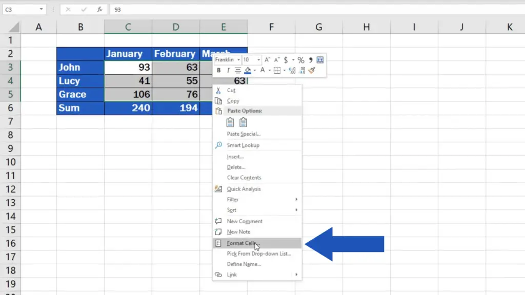
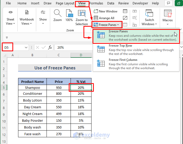
Web select a cell in the first column directly below the rows you want to freeze. Choose the freeze panes option from the menu. Navigate to the view tab and locate the window group. You can see a black line under the first row which signals that the row is now locked. Freeze only the first column. In case you want to lock multiple rows, you can do so by highlighting them before proceeding to the next step. In the above example, cell a4 is selected, which means rows 1:3 will be frozen in place.
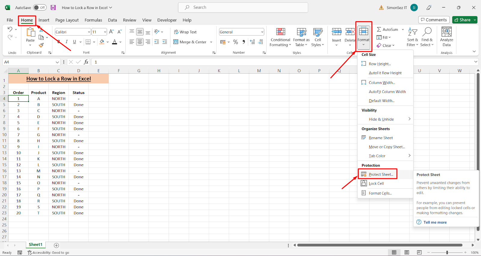
How to Lock Cells in Excel
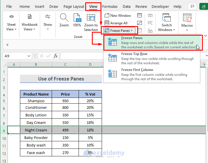
Select view > freeze panes > freeze panes. Go to the view tab on the ribbon. Select the cell below the rows and to the right of the columns you want to keep visible when you scroll. To do this, click on the row number located on the left of the worksheet. You can see.
How to Lock Cells in Excel
Web freeze the first two columns. Click on the freeze panes command. In case you want to lock multiple rows, you can do so by highlighting them before proceeding to the next step. Navigate to the view tab and locate the window group. Go to the view tab on the ribbon. Select the cell below.
How to Lock Rows in Excel (6 Easy Methods) ExcelDemy
Select view > freeze panes > freeze panes. Click on the freeze panes command. Freeze multiple rows or columns. Select the cell below the rows and to the right of the columns you want to keep visible when you scroll. Web if you want the row and column headers always visible when you scroll through.

How to Lock a Row in Excel YouTube
This will highlight the entire row. Navigate to the view tab and locate the window group. This will lock only the top row. Web select a cell in the first column directly below the rows you want to freeze. How to freeze multiple rows in excel. In the above example, cell a4 is selected, which.
How to Lock Cells in Excel
Navigate to the view tab and locate the window group. Web select a cell in the first column directly below the rows you want to freeze. Choose the freeze panes option from the menu. Select the row below the last row you want to freeze. Select the cell below the rows and to the right.

How to Lock Rows in Excel (6 Easy Methods) ExcelDemy
Freeze multiple rows or columns. Click on the freeze panes command. How to freeze multiple rows in excel. In case you want to lock multiple rows, you can do so by highlighting them before proceeding to the next step. Freezing the selected row (s) Select the row below the last row you want to freeze..

How to Lock Cells in Excel (with Pictures) wikiHow
Tap view > freeze panes, and then tap the option you need. Select the cell below the rows and to the right of the columns you want to keep visible when you scroll. Freeze multiple rows or columns. Choose the freeze panes option from the menu. Go to the view tab on the ribbon. This.
How to Lock Rows in Excel (6 Easy Methods) ExcelDemy
Go to the view tab on the ribbon. Freeze only the first column. Navigate to the view tab and locate the window group. This will lock only the top row. Web the first step in locking a row in excel is to select the row or rows you want to freeze. Tap view > freeze.
How to Lock a Row in Excel? 4 Useful Ways
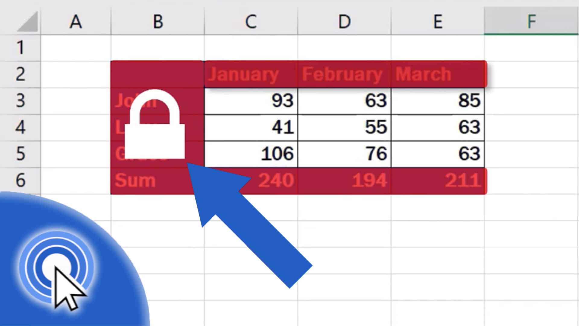
Web the first step in locking a row in excel is to select the row or rows you want to freeze. Click on the freeze panes command. If we scroll down, we can see that the top row is frozen. This will lock the first row of your worksheet, ensuring that it remains visible when.
How to lock cell in Excel steps on how to go about it
Select the row below the last row you want to freeze. In the above example, cell a4 is selected, which means rows 1:3 will be frozen in place. Web select a cell in the first column directly below the rows you want to freeze. Go to the view tab on the ribbon. Select view >.
How Do You Lock A Row In Excel You can see a black line under the first row which signals that the row is now locked. Select the cell below the rows and to the right of the columns you want to keep visible when you scroll. To do this, click on the row number located on the left of the worksheet. Web freeze the first two columns. Freezing the selected row (s)
How To Freeze Multiple Rows In Excel.
Freeze multiple rows or columns. Web the first step in locking a row in excel is to select the row or rows you want to freeze. This will lock the first row of your worksheet, ensuring that it remains visible when you browse through the remainder of it. To do this, click on the row number located on the left of the worksheet.
Web Freeze The First Two Columns.
You can see a black line under the first row which signals that the row is now locked. Go to the view tab on the ribbon. Select the row below the last row you want to freeze. Choose the freeze panes option from the menu.
This Will Highlight The Entire Row.
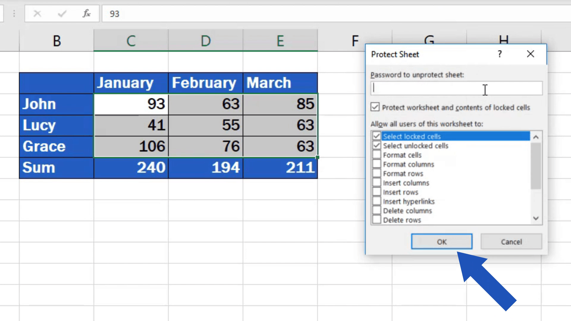
In case you want to lock multiple rows, you can do so by highlighting them before proceeding to the next step. Web if you want the row and column headers always visible when you scroll through your worksheet, you can lock the top row and/or first column. If we scroll down, we can see that the top row is frozen. Freezing the selected row (s)
Click On The Freeze Panes Command.
Navigate to the view tab and locate the window group. Tap view > freeze panes, and then tap the option you need. Go to the view tab. Select view > freeze panes > freeze panes.